How To Show Negative Percentages In Parentheses In Excel
You can do this on the Modeling tab of the desktop. In the Type box enter the following format.
7 Amazing Excel Custom Number Format Tricks You Must Know

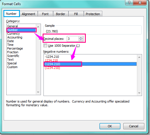
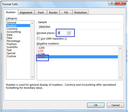
Enter 0 in the Decimal placesbox to avoid decimals.
How to show negative percentages in parentheses in excel. Add Parenthesis to Negative Percentages. Open your file in Excel. Add Brackets.
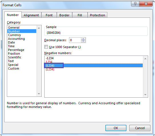
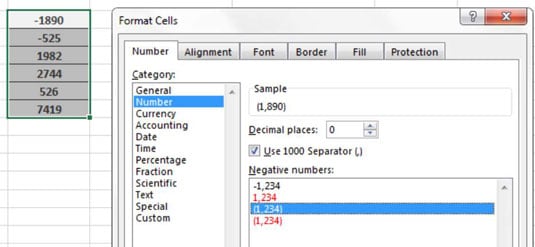
On the Home tab click Format Format Cells. Select the Number tab and from Category select Number. When a formula returns a negative percentage the result is formatted as -49.
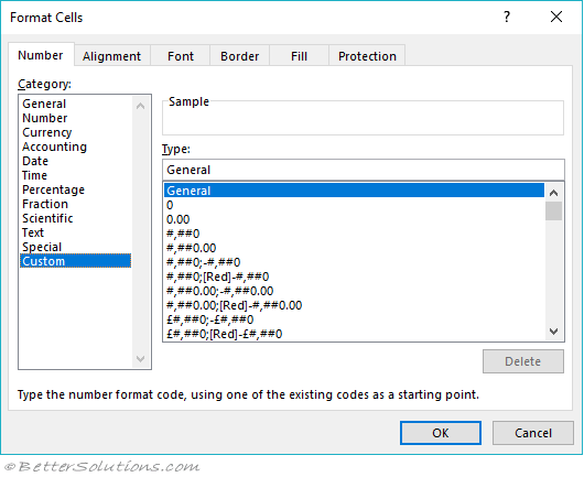
For example you may want to show an expense of 5000 as 5000 or -5000. In the Format Cells box in the Category list click Custom. Change it to a decimal format then Custom.
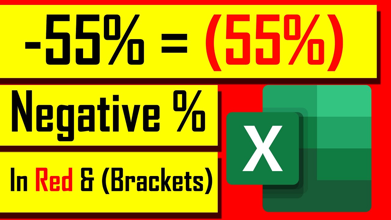
Use to display number or nothing For instance if you have the number 123. Hi Right click on the cell you want to format choos format cells choos the. Negative Percentage in Parenthesis instead of with - sign.
You can add percentages like any other number. In this Advanced Excel tutorial you are going to learn ways. Is there any format in Excel 2002 that allows for it to be formatted 49.
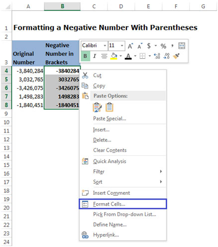
Enter the custom format above. Mark negative percentage in red by creating a custom format. Use your mouse to select the cells of the spreadsheet.
You can learn more about these regional settings on Microsofts website. In accounting and financial models sometimes you will want to show negative numbers in brackets and in red color. Click on Format Cells orPress Ctrl1 on the keyboard to open the Format Cells dialog box.
Follow these steps to display parentheses around negative numbers. How to Add Percentages Together. Number tab choos custom enter in the Type text box.
Add Brackets Minus Sign Mark Red All Negative PercentagesIn this Excel tutorial you ar. In the formula bar type sum without quotes and then click the first result the sum formula which adds all numbers in a range of cells. Now select the cells to which to apply this formatting.
If you want a minus sign in front of your negative financial values rather than enclosing them in parentheses select the Currency format on the Number Format drop-down menu or on the Number tab of the Format Cells dialog box. In the Negative Numbers box select the last option as highlighted. To so so follow the following steps.
Use the custom format. From the Number sub menu select Custom. Click on the Home tab on the top of the window and click Format button in the cells section and select format cells option.
Use 0 to display number or 0 if empty. You can also change the font color to red. Right click on the cell that you want to format.
If youre using Excel and negative numbers arent displaying with parentheses you can change the way negative numbers are displayedBut if that doesnt work or if the parentheses option 123410 isnt available its likely because an operating system setting isnt set properly. You can create a custom format to quickly format all negative percentage in red in Excel. How to display negative numbers in brackets in excel.
If youre using a Mac make sure you use the App Store and update to the latest version of macOS. Select the modeling tab. Select the cells which have the negative percentage you want to mark in red.
Select the cells right click on the mouse. In this example were going to click and highlight cell C3. Choose a cell to display the sum of your two percentages.
You can always use a custom format FormatCellsNumberCustom Type. In parentheses you can choose red or black In the UK and many other European countries youll typically be able to set negative numbers to show in black or red and with or without a minus sign in both colors but have no option for parentheses. 000 hope this will work for you.
There is a more in depth article here about custom number formats. I have been able to format single cells to display negative percents Budget to Actual hours but I cannot copy the formatting to cells with positive percents without eliminating the format style I want. To select multiple cells hold down the Ctrl key as you.
Select the cell or cells that contain negative percentages. Right click the selected cells and select Format Cells in the right-clicking menu. Click on Format Cells.
I need to display with the parenthesis 136for negative results. Code to customize numbers in Excel.
Displaying Negative Numbers In Parentheses Excel

How To Display Negative Percentages In Red Within Brackets In Excel Youtube
Excel Formatting Custom
Formatting A Negative Number With Parentheses In Microsoft Excel
Formatting A Negative Number With Parentheses In Microsoft Excel

Kb40241 The Negative Percentage Values In A Graph Report Are Displayed Outside The Parenthesis In Microstrategy Web And Developer 10 X
Formatting A Negative Number With Parentheses In Microsoft Excel
Unable To Format Negative Values In Excel Using Parentheses Microsoft Community
Excel Reports Custom Number Formatting Dummies
Displaying Negative Numbers In Parentheses Excel

How To Display Negative Numbers In Brackets In Excel
How To Display Negative Values In Red And Within Brackets In Excel Youtube

How To Get Parentheses For Negative Numbers In Excel Mac Lasopacolumbus

Displaying Negative Numbers In Parentheses Excel

Formatting A Negative Number With Parentheses In Microsoft Excel
Accounting Format Negative Numbers Microsoft Community
Displaying Negative Numbers In Parentheses Excel

Formatting A Negative Number With Parentheses In Microsoft Excel
Excel Format Negative Percentage Parentheses Architectlasopa

